반응형
신경망 학습 절차
전제
신경망에는 적응 가능한 가중치와 편향이 있고, 이 가중치와 편향을 훈련 데이터에 적응하도록 조정하는 과정을 '학습'이라고 합니다. 신경망 학습은 다음과 같이 4단계로 수행합니다.
1단계 - 미니배치
훈련 데이터 중 일부를 무작위로 가져옵니다. 이렇게 선별한 데이터를 미니배치라 하며, 그 미니배치의 손실 함수 값을 줄이는 것이 목표입니다.
2단계 - 기울기 산출
미내배치의 손실 함수 값을 줄이기 위해 각 가중치 매개변수의 기울기를 구합니다. 기울기는 손실 함수의 값을 가장 적게 하는 방향을 제시합니다.
3단계 - 매개변수 갱신
가중치 매개변수를 기울기 방향으로 아주 조금 갱신합니다.
4단계 - 반복
1 ~ 3단계를 반복합니다.
이것이 신경망 학습이 이뤄지는 순서입니다. 이는 경사 하강법으로 매개변수를 갱신하는 방법이며, 이때 데이터를 미내배치로 무작위로 선정하기 때문에 확률적 경사 하강법(SGD)라고 부릅니다. 대부분의 딥러닝 프레임워크는 확률적 경사 하강법의 영어 머리글자를 딴 SGD라는 함수로 이 기능을 구현하고 있습니다.
2층 신경망 클래스 구현하기
import sys, os, numpy as np
sys.path.append(os.pardir)
from common.functions import *
from common.gradient import numerical_gradient

class TwoLayerNet:
    def __init__(self, input_size, hidden_size, output_size, weight_init_std=0.01):
        self.params = {}
        self.params['W1'] = weight_init_std * np.random.randn(input_size, hidden_size)
        self.params['b1'] = np.zeros(hidden_size)
        self.params['W2'] = weight_init_std * np.random.randn(hidden_size, output_size)
        self.params['b2'] = np.zeros(output_size)
	#__init__함수는 초기화를 진행합니다. 신경망을 구성하는 매개변수를 딕셔너리를 사용했습니다.
    #각 가중치와 편향을 초기화했습니다.

    def predict(self, x):
        W1, W2 = self.params['W1'], self.params['W2']
        b1, b2 = self.params['b1'], self.params['b2']

        a1 = np.dot(x, W1) + b1
        z1 = sigmoid(a1)
        a2 = np.dot(z1, W2) + b2
        y = sigmoid(a2)

        return y
    #predict함수는 예측(추론)을 수행합니다. 이때 인수x는 이미지 데이터입니다.

    def loss(self, x, t):
        y = self.predict(x)

        return cross_entropy_error(y, t)
    //loss함수는 예측된 값과 실제 레이블간의 손실 함수를 계산합니다.

    def accuracy(self, x, t):
        y = self.predict(x)
        y = np.argmax(y, axis=1)
        t = np.argmax(t, axis=1)

        accuracy = np.sum(y == t) / float(x.shape[0])

        return accuracy
    //accuracy함수는 정확도를 구합니다

    def numerical_gradient(self, x, t):
        loss_W = lambda W: self.loss(x, t)

        grads = {}
        grads['W1'] = numerical_gradient(loss_W, self.params['W1'])
        grads['b1'] = numerical_gradient(loss_W, self.params['b1'])
        grads['W2'] = numerical_gradient(loss_W, self.params['W2'])
        grads['b2'] = numerical_gradient(loss_W, self.params['b2'])

        return grads
    //numerical_gradient함수는 기울기를 구합니다.
각 주석을 달았지만 이해가 되지 않는 분은 댓글 남겨주세요. 구현한 신경망을 확인해보겠습니다.
net = TwoLayerNet(input_size=784, hidden_size=100, output_size=10)
print(net.params['W1'].shape)
print(net.params['b1'].shape)
print(net.params['W2'].shape)
print(net.params['b2'].shape)

[출력]
(784, 100)
(100,)
(100, 10)
(10,)
x = np.random.rand(100, 784)
y = net.predict(x)
y.shape
[출력]
(100, 10)
미니배치 학습 구현하기
import numpy as np
from dataset.mnist import load_mnist
from two_layer_net import TwoLayerNet

(x_train, t_train), (x_test, t_test) = load_mnist(normalize=True, one_hot_label=True)

train_losss_list = []

iters_num = 100
train_size = x_train.shape[0]
batch_size = 100
learning_rate = 0.1

network = TwoLayerNet(input_size=784, hidden_size=50, output_size=10)

for i in range(iters_num):
    batch_mask = np.random.choice(train_size, batch_size)
    #train_size중에 batch_size만큼 무작위로 골라
    x_batch = x_train[batch_mask]
    t_batch = t_train[batch_mask]

    grad = network.numerical_gradient(x_batch, t_batch)

    for key in ('W1', 'b1', 'W2', 'b2'):
        network.params[key] -= learning_rate * grad[key]

    loss = network.loss(x_batch, t_batch)
    train_losss_list.append(loss)
시험 데이터로 평가하기
import sys, os
sys.path.append(os.pardir)  # 부모 디렉터리의 파일을 가져올 수 있도록 설정
import numpy as np
import matplotlib.pyplot as plt
from dataset.mnist import load_mnist
from two_layer_net import TwoLayerNet

# 데이터 읽기
(x_train, t_train), (x_test, t_test) = load_mnist(normalize=True, one_hot_label=True)

network = TwoLayerNet(input_size=784, hidden_size=50, output_size=10)

# 하이퍼파라미터
iters_num = 10000  # 반복 횟수를 적절히 설정한다.
train_size = x_train.shape[0]
batch_size = 100   # 미니배치 크기
learning_rate = 0.1

train_loss_list = []
train_acc_list = []
test_acc_list = []

# 1에폭당 반복 수
iter_per_epoch = max(train_size / batch_size, 1)

for i in range(iters_num):
    # 미니배치 획득
    batch_mask = np.random.choice(train_size, batch_size)
    x_batch = x_train[batch_mask]
    t_batch = t_train[batch_mask]

    # 기울기 계산
    #grad = network.numerical_gradient(x_batch, t_batch)
    grad = network.gradient(x_batch, t_batch)

    # 매개변수 갱신
    for key in ('W1', 'b1', 'W2', 'b2'):
        network.params[key] -= learning_rate * grad[key]

    # 학습 경과 기록
    loss = network.loss(x_batch, t_batch)
    train_loss_list.append(loss)

    # 1에폭당 정확도 계산
    if i % iter_per_epoch == 0:
        train_acc = network.accuracy(x_train, t_train)
        test_acc = network.accuracy(x_test, t_test)
        train_acc_list.append(train_acc)
        test_acc_list.append(test_acc)
        print("train acc, test acc | " + str(train_acc) + ", " + str(test_acc))

# 그래프 그리기
markers = {'train': 'o', 'test': 's'}
x = np.arange(len(train_acc_list))
plt.plot(x, train_acc_list, label='train acc')
plt.plot(x, test_acc_list, label='test acc', linestyle='--')
plt.xlabel("epochs")
plt.ylabel("accuracy")
plt.ylim(0, 1.0)
plt.legend(loc='lower right')
plt.show()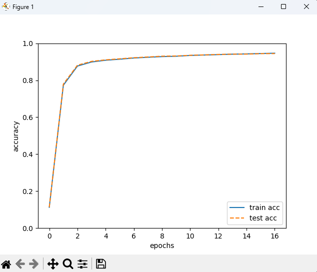
반응형
'ML & DL > 밑바닥부터 시작하는 딥러닝' 카테고리의 다른 글
| [파이썬 딥러닝] 활성화 함수 계층 구현하기 (0) | 2023.03.29 |
|---|---|
| [파이썬 딥러닝]순전파와 역전파 기초 (0) | 2023.03.28 |
| [파이썬 딥러닝] 수치 미분 (0) | 2023.03.22 |
| [파이썬 딥러닝] 신경망 학습 (0) | 2023.03.16 |
| [파이썬 딥러닝] 신경망 (0) | 2023.03.14 |


